
First Order System
First order system transfer function equals to:
H(s) = K/(s-p1)
Low pass RC filter is an example of a first order system with one pole: p = -1/(R*C)
Impulse response is determined via Inverse Laplace transform:
h(t) = K*exp(p*t)
Gain and Phase Margins
Gain margin is the negative of open loop dB gain at 180 degree phase shift.
Phase margin is the difference between 0 dB open loop gain phase and -180 degrees.
Gain and phase margins are determined by plotting system transfer functions/Bode plots (en.wikipedia.org/wiki/Bode_plot).
Example
System transfer function:
Open Loop Gain = A0(s) =K/((1+s/w0)*(1+s/w0)*(1+s/w0)) where f0 = 10 Hz
System feedback factor: Beta = 1
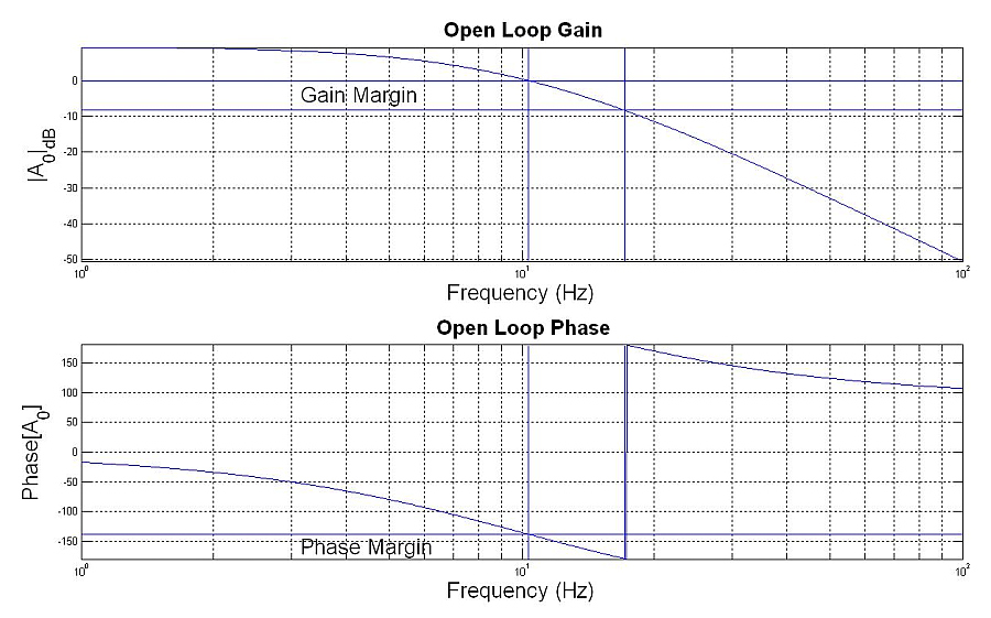
The system will become a phase shift oscillator if phase and gain margins fall below zero, satisfying the following conditions for oscillations:
Loop Gain |A0*Beta| > 1 and phase[A0*Beta] = -180
% Matlab code
% Gain and Phase Margins
clear all;close all
N=1000;f=logspace(0,2,N);w=2*pi*f;s=j*w;w0=2*pi*10;
H=3./((1+s/w0).*(1+s/w0).*(1+s/w0));
f0dB=max(find(20*log10(abs(H))>0));
f180=min(find((angle(H)/pi*180)<-179));
gainmargin=abs(20*log10(abs(H(f180))));
phasemargin=(angle(H(f0dB))-angle(H(f180)))/pi*180;
disp(['Gain Margin = ' num2str(gainmargin) ' dB'])
disp(['Phase Margin = ' num2str(phasemargin) ' degrees'])
subplot(2,1,1);semilogx(f,20*log10(abs(H)));grid on;axis tight
hold on;line([f(f180(1)) f(f180(1))],[min(20*log10(abs(H))) max(20*log10(abs(H)))])
hold on;line([f(f0dB(1)) f(f0dB(1))],[min(20*log10(abs(H))) max(20*log10(abs(H)))])
hold on;line([f(1) f(N)],[0 0])
hold on;line([f(1) f(N)],[-gainmargin -gainmargin])
text(f(round(N/4)),round(-gainmargin/2),'Gain Margin','fontsize',20)
title('\bf Open Loop Gain','fontsize',20)
xlabel('Frequency (Hz)','fontsize',20);ylabel('|A_0|_d_B','fontsize',20)
subplot(2,1,2);semilogx(f,180/pi*angle(H));grid on;axis tight
hold on;line([f(f180(1)) f(f180(1))],[min(180/pi*angle(H)) max(180/pi*angle(H))])
hold on;line([f(f0dB(1)) f(f0dB(1))],[min(180/pi*angle(H)) max(180/pi*angle(H))])
hold on;line([f(1) f(N)],[angle(H(f0dB))/pi*180 angle(H(f0dB))/pi*180])
text(f(round(N/4)),-180+round(phasemargin/2),'Phase Margin','fontsize',20)
title('\bf Open Loop Phase','fontsize',20)
xlabel('Frequency (Hz)','fontsize',20);ylabel('Phase[A_0]','fontsize',20)
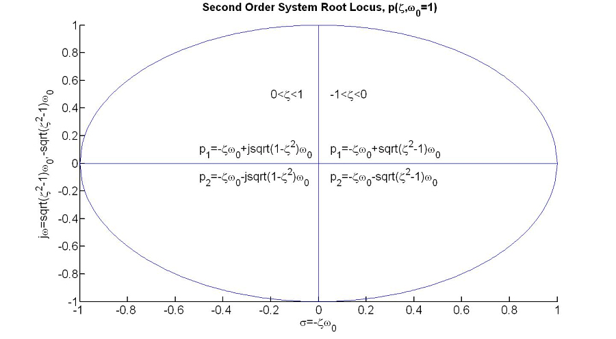
Root Locus
Root locus is a plot of system poles in terms of damping ratio zeta.
Example
Define second order system transfer function:
H(s) = K/((s/w0)^2+2*zeta*s/w0+1)
H(s) = K/((s-p1)*(s-p2))
Gain is infinite for s = p1,p2.
Second order system poles equal to:
p1,2 = -zeta*w0 + sqrt(zeta^2 - 1)*w0, = -zeta*w0 - sqrt(zeta^2 - 1)*w0
where: zeta = damping ratio
thus p2 = conj(p1)
Assuming w0 = 1 rad/s we get root locus plot:
Underdamped system transient impulse response:
h(t) = 2*Re[A*exp(p1*t)] = 2*|A|*exp(-zeta*w0*t)*cos(w0*sqrt(1-zeta^2)*t+phase(A))
where: A = |A|*exp(j*phase(A))
% Matlab code
% Root Locus
clear all;close all
figure;A=axes;set(A,'FontSize',20,'LineWidth',2);hold on
zeta=linspace(0,1,100);w0=1;
plot(-zeta.*w0,w0.*sqrt(1-zeta.^2));hold on;plot(-zeta.*w0,-w0.*sqrt(1-zeta.^2))
zeta=linspace(-1,0,100);p=-zeta.*w0+sqrt((zeta.^2)-1).*w0;
plot(real(p),imag(p));hold on;plot(real(conj(p)),imag(conj(p)))
text(0.05,0.1,'p_1=-\zeta\omega_0+sqrt(\zeta^2-1)\omega_0','fontsize',20)
text(-0.5,0.1,'p_1=-\zeta\omega_0+jsqrt(1-\zeta^2)\omega_0','fontsize',20)
line([-1 1],[0 0])
text(0.05,-0.1,'p_2=-\zeta\omega_0-sqrt(\zeta^2-1)\omega_0','fontsize',20)
text(-0.5,-0.1,'p_2=-\zeta\omega_0-jsqrt(1-\zeta^2)\omega_0','fontsize',20)
text(-0.2,0.5,'0<\zeta<1','fontsize',20)
line([0 0],[-1 1])
text(0.05,0.5,'-1<\zeta<0','fontsize',20)
title('\bf Second Order System Root Locus, p(\zeta,\omega_0=1)','fontsize',20)
xlabel('\sigma=-\zeta\omega_0','fontsize',20);ylabel('j\omega=sqrt(\zeta^2-1)\omega_0,-sqrt(\zeta^2-1)\omega_0','fontsize',20)